Optimizing the energy network

Once the energy system has been defined as an object of the EnergyNetworkIndiv class or the EnergyNetworkGroup class and the model components (and parameters) have been set from the input excel file, the network object could then be optimized:

envImpact, capacitiesTransformers, capacitiesStorages = network.optimize(solver='gurobi',
                                                                       envImpactlimit=envImpactlimit,
                                                                       clusterSize=clusterSize,
                                                                       options=optimizationOptions,
                                                                       mergeLinkBuses=mergeLinkBuses)

The first parameter solver specifies the name of solver to be used for optimization. solver could take the values gurobi, cbc, cplex or glpk. envImpactlimit denotes the maximum limit for environmental impact. This parameter becomes relevant in case of multi-objective optimization and would be described in the later sections. For single-objective optimization set this parameter to a significantly high value which would never be reached (For example: 10^6). clusterSize is the parameter related to clustered days (if defined). This is an optional parameter and is required only if clustered days are used. options specifies the command line parameters to be passed to the selected solver. This parameter is described further in the following section. The mergeLinkBuses defines whether or not the buses of the different buildings should be merged (set to False if not given). The optimize function returns the environmental impact of the optimized energy model, the capacities selected for energy transformers (or converters such as CHP, heat pump, etc.) and for the storages in the optimized energy network model.

Optimization options

The options parameter of the optimize function allows passing command line options to the solver. The optimization options could be passed as a dictionary indexed by the solver name. For example:

# solver specific command line options
optimizationOptions = {
    "gurobi": {
        "BarConvTol": 0.5,
        # The barrier solver terminates when the relative difference between the primal and dual objective values is less than the specified tolerance (with a GRB_OPTIMAL status)
        "OptimalityTol": 1e-4,
        # Reduced costs must all be smaller than OptimalityTol in the improving direction in order for a model to be declared optimal
        "MIPGap": 1e-2,
        # Relative Tolerance between the best integer objective and the objective of the best node remaining
        "MIPFocus": 2
        # 1 feasible solution quickly. 2 proving optimality. 3 if the best objective bound is moving very slowly/focus on the bound
        # "Cutoff": #Indicates that you aren't interested in solutions whose objective values are worse than the specified value., could be dynamically be used in moo
    },
    "cbc": {"tee": False}
}

The options for a new solver could be added as a new item in this dictionary in the form:

solver_name:{option_name: option_value}

where solver_name specifies the name of the solver, option_name and option_value are the name and value, respectively of the command line option.

For more details on the different command line options which could be passed to the solver, we recommend you to have a look at the documentation of the respective solver.

Dispatch optimization

The dispatch optimization is an option that enables to optimize the size of the used technologies but does not decide whether to use them or not (it supposes that they are already installed). In this way, it is opposite to the investment optimization where the different available technologies are compared and then selected based on the optimized scenario.

Single-objective optimization

Single-objective optimization can be performed easily by calling the optimize function of the EnergyNetworkIndiv or EnergyNetworkGroup class once the energy network has been defined. The optimization problem and the energy network should be defined using the input excel file. The target for single-objective optimization could be specified at this stage as a parameter passed in the setFromExcel function:

network.setFromExcel(inputExcelFilePath, numberOfBuildings, clusterSize, opt, mergeLinkBuses, dispatchMode)

The parameter dispatchMode is used to decide whether or not the dispatch optimization is applied (set to False if not given). The parameter opt could be set to either 'costs' or 'env' for optimization based on cost or environmental impact, respectively. The respective data related to costs/environmental impact of the energy resources and the available energy conversion and storage technologies should be given in the appropriate sections of the input excel file.

For more details on the setFromExcel function and the structure of the input excel file, have a look at Defining an energy network.

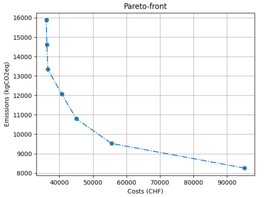
Multi-objective optimization

Multi-objective optimization can be performed as multiple single objective optimizations. At present, the two supported target objectives are 'costs' (total cost) and 'env' (environmental emission). The first optimization would then be for cost minimization and the second for the minimization of emissions, which would give the two extremes i.e. cost-optimum solution and environmental optimum solution. And then, more solutions are obtained between the cost and environmental optimum, these optimizations are a minimization of the cost subject to a constraint on the environmental criteria (epsilon constraint method). The speed of optimization would be greatly affected by the number of optimizations to be performed.

The results from multi-objective optimization can be visualized using a pareto front.

For more information on how to work with multi-objective optimization go through the example.

Clustering

Clustering feature allows the users to improve the optimization speed by specifying a set of dates which could be considered representative of the whole year (or the entire duration of the analysis). For example: four typical days could be selected , one representing each season, and optihood would then provide the optimal design plan of the energy network based on these days. Since the time resolution of the optimization problem would be much lower than simulating the whole year, the speed of optimization is much faster when clustering is used.

Any clustering method (for example K-means clustering) can be chosen by the user and the results could be fed to optihood for faster optimization. Note that in optihood one could use the results from clustering (which is to be done independently) but the implementation of the clustering method itself is not a part of the optihood framework. The following results are required from the clustering algorithm:

Number of clusters
Days of year representing each cluster
Number of days in each cluster

In order to use the clustering feature, first a dictionary containing one item for each cluster, where keys and values are the cluster’s representative date and number of days, respectively, should be defined:

cluster = {"2018-07-30": 26,
           "2018-02-03": 44,
           "2018-07-23": 32,
           "2018-09-18": 28,
           "2018-04-15": 22,
           "2018-10-01": 32,
           "2018-11-04": 32,
           "2018-10-11": 37,
           "2018-01-24": 15,
           "2018-08-18": 26,
           "2018-05-28": 23,
           "2018-02-06": 48}

Here, the days of the year have been represented using 12 clusters, where the first cluster consists of 26 days and is represented by the date 30 June 2018.

This dictionary should be passed in the setFromExcel and optimize functions of the EnergyNetwork class:

# set a time period for the optimization problem according to the number of clusers
network = EnergyNetwork(pd.date_range("2018-01-01 00:00:00", "2018-01-12 23:00:00", freq="60min"), temperatureSH, temperatureDHW)

# pass the dictionary defining the clusters to setFromExcel function
network.setFromExcel("scenario.xls", numberOfBuildings=4, clusterSize=cluster, opt="costs")

# pass the dictionary defining the clusters to optimize function
envImpact, capacitiesTransformers, capacitiesStorages = network.optimize(solver='gurobi', clusterSize=cluster)

Note that the time period would need to be adjusted to include the timesteps corresponding to 12 days (12 x 24 = 288 timesteps if hourly resolution is considered). Try the example on selective days clustering for a better grasp.